Accuracy Metrics
Summary
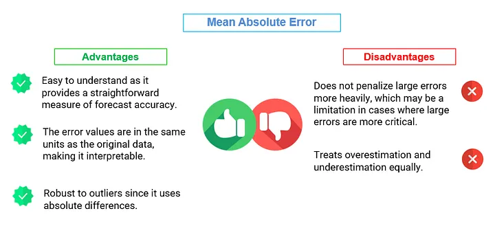
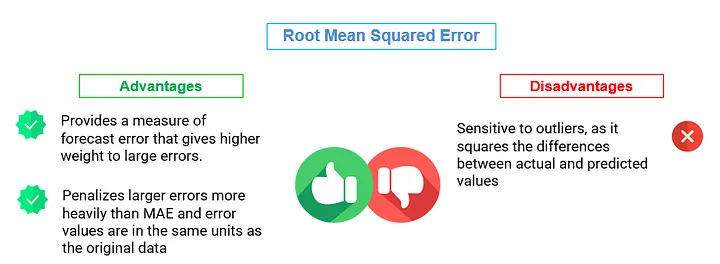
- Use MAE (Mean Absolute Error) and RMSE (Root Mean Squared Error) when you want to measure the magnitude of errors and need a metric that is easy to interpret. RMSE is preferred when larger errors should be penalized more heavily.
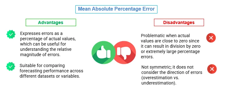
- Use MAPE (Mean Absolute Percentage Error) and SMAPE (Symmetric Mean Absolute Percentage Error) when you want to express errors as percentages of actual values and need a metric that is suitable for comparing forecast performance across different datasets.
- Use MDAPE (Median Absolute Percentage Error) when dealing with time series data that may have outliers or extreme values. MDAPE is robust to outliers because it calculates the median of the absolute percentage errors.
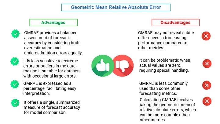
- Use GMRAE (Geometric Mean Relative Absolute Error) when you want to compare forecast performance across different time series with varying scales. GMRAE provides a balanced measure of forecast accuracy across multiple forecasts.
Mean Absolute Error (MAE)
The Mean Absolute Error (MAE) is a commonly used metric for measuring the accuracy of predictions or forecasts. It quantifies the average absolute difference between the predicted or forecasted values and the actual values. The formula for calculating MAE is as follows:
MAE = (1 / n) * Σ |actual — forecast|
Where:
MAE is the Mean Absolute Error.
n is the number of data points (samples).
Σ represents the sum over all data points.
| actual — forecast | is the absolute difference between the actual value and the forecasted value for each data point. |
Let’s find the MAE for our data.
from sklearn.metrics import mean_absolute_error
# Calculate Mean Absolute Error (MAE)
mae = mean_absolute_error(final_test_data['y'], final_test_data['AutoARIMA'])
# Print MAE
print(f"Mean Absolute Error (MAE): {mae:.4f}")
Output :- Mean Absolute Error (MAE): 2.8489
MAE of 2.8489 indicates that, on average, our forecasts are off by about 2.8489 units from the actual values. A lower MAE suggests better accuracy, while a higher MAE indicates less accurate forecasts.
Root Mean Squared Error (RMSE)
The Root Mean Squared Error (RMSE) is another widely used metric for measuring the accuracy of predictions or forecasts. RMSE quantifies the average magnitude of errors between the predicted or forecasted values and the actual values, giving more weight to larger errors. It’s an important metric, especially when larger errors are of greater concern. The mathematical expression for calculating RMSE is as follows:
RMSE = √((1 / n) * Σ(actual — forecast)²)
Where:
RMSE is the Root Mean Squared Error.
n is the number of data points (samples).
Σ represents the sum over all data points.
(actual — forecast)² is the squared difference between the actual value and the forecasted value for each data point.
Let us check the RMSE for this data:
from sklearn.metrics import mean_squared_error
# Calculate the Root Mean Squared Error (RMSE)
rmse = mean_squared_error(final_test_data['y'], final_test_data['AutoARIMA'],
                          squared=False)

# Print the RMSE
print(f"Root Mean Squared Error (RMSE): {rmse:.4f}")
Output :- Root Mean Squared Error (RMSE): 3.8863
RMSE quantifies the average magnitude of the errors. In this case, an RMSE of 3.8863 suggests that, on average, the forecasts are off by about 3.8863 units from the actual values.
Mean Absolute Percentage Error (MAPE)
The Mean Absolute Percentage Error (MAPE) is a metric used to measure the accuracy of predictions or forecasts as a percentage of the actual values. It quantifies the average percentage difference between the predicted or forecasted values and the actual values. The mathematical expression for calculating MAPE is as follows:
MAPE = (1 / n) * Σ(|(actual — forecast) / actual|) * 100%
Where:
n is the number of data points (samples).
Σ represents the sum over all data points.
| (actual — forecast) / actual | is the absolute percentage difference between the actual value and the forecasted value for each data point. |
The result is multiplied by 100% to express the error as a percentage.
Let us find the MAPE for our data:
import numpy as np

def mean_absolute_percentage_error(y_true, y_pred):
    """
    Calculate Mean Absolute Percentage Error (MAPE)

    Args:
    y_true: array-like of shape (n_samples,) - True values
    y_pred: array-like of shape (n_samples,) - Predicted values

    Returns:
    mape: float - Mean Absolute Percentage Error
    """
    y_true, y_pred = np.array(y_true), np.array(y_pred)
    result = np.mean(np.abs((y_true - y_pred) / y_true)) * 100

    # Check for infinity and replace with 0
    if np.isinf(result):
        return 0.0
    return mape


  import numpy as np
  mape = np.mean(np.abs((final_test_data['y'] - final_test_data['AutoARIMA'])/ final_test_data['y'])) * 100
  print(f"Mean Absolute Percentage Error (MAPE): {mape:.4f}")
Output :- Mean Absolute Percentage Error (MAPE): 2.6810
A MAPE of 2.6810 suggests that, on average, your forecasts deviate by about 2.6810% from the actual values. A lower MAPE indicates better accuracy, while a higher MAPE suggests less accurate forecasts.
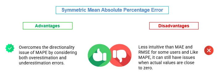
Symmetric Mean Absolute Percentage Error (SMAPE)
The Symmetric Mean Absolute Percentage Error (SMAPE) is a metric used for measuring the accuracy of predictions or forecasts in time series analysis. It’s particularly useful when you want to assess forecast accuracy while considering both overestimation and underestimation errors. SMAPE calculates the percentage difference between predicted or forecasted values and actual values, but it symmetrically treats overestimation and underestimation errors. The mathematical expression for calculating SMAPE is as follows:
SMAPE = (1 / n) * Σ(2 * |actual — forecast| / (|actual| + |forecast|)) * 100%
Where:
SMAPE is the Symmetric Mean Absolute Percentage Error, expressed as a percentage.
n is the number of data points (samples).
Σ represents the sum over all data points.
| actual — forecast | is the absolute difference between the actual value and the forecasted value for each data point. | actual | and | forecast | are the absolute values of the actual and forecasted values, respectively. |
The result is multiplied by 100% to express the error as a percentage.
Let us check the SMAPE for our data:
import numpy as np
from sklearn.metrics import mean_absolute_percentage_error

y_true = np.array([100, 200, 300, 400, 0])
y_pred = np.array([110, 190, 310, 420, 0])

# Mask to exclude zero values in y_true
mask = y_true != 0

mape = mean_absolute_percentage_error(y_true[mask], y_pred[mask]) * 100
print(f"MAPE: {mape}%")


  smape = np.mean((np.abs(final_test_data['y'] - final_test_data['AutoARIMA']) /((np.abs(final_test_data['y'] +np.abs(final_test_data['AutoARIMA'])) / 2))) * 100
  print(f"Symmetric Mean Absolute Percentage Error (SMAPE): {smape:.4f}")
Output :- Symmetric Mean Absolute Percentage Error (SMAPE): 2.6773
SMAPE of 2.6773 suggests that, on average, our forecasts deviate by about 2.6773% from the actual values in a symmetric manner. A lower SMAPE indicates better accuracy, while a higher SMAPE suggests less accurate forecasts.
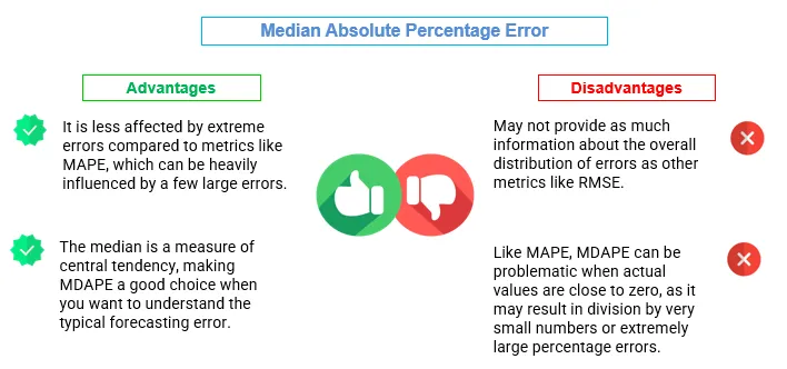
Median Absolute Percentage Error (MDAPE)
MDAPE stands for Median Absolute Percentage Error. It is a performance metric used to evaluate the accuracy of forecasts in time series analysis. MDAPE is similar to the Mean Absolute Percentage Error (MAPE), but instead of taking the mean of the absolute percentage errors, it takes the median. This makes MDAPE less sensitive to outliers than MAPE.
The formula for calculating MDAPE is as follows:
MDAPE = Median(|(Actual — Forecast) / Actual|) * 100%
Where:
Actual represents the actual values or observations in the time series.
Forecast represents the corresponding forecasted values.
MDAPE is expressed as a percentage, and it measures the median percentage difference between the actual and forecasted values. It is particularly useful when dealing with time series data that may have extreme values or outliers because it focuses on the middle value of the distribution of percentage errors.
Let’s check how MDAPE looks for our data:
mdape = np.median(np.abs((final_test_data['y'] - final_test_data['AutoARIMA'])/ final_test_data['y']))*100
print(f"Median Absolute Percentage Error (MDAPE): {mdape:.4f}")
Output :- Median Absolute Percentage Error (MDAPE): 1.7398
An MDAPE of 1.7398 indicates that, on average, forecasting errors are relatively low, comprising approximately 1.7398% of actual values.
Geometric Mean Relative Absolute Error (GMRAE)
The Geometric Mean Relative Absolute Error (GMRAE) is a metric used to assess the accuracy of predictions or forecasts in time series analysis. It takes the geometric mean of the relative absolute errors, providing a single aggregated measure of forecast accuracy. GMRAE is particularly useful when you want to consider both overestimation and underestimation errors. Here’s the mathematical formula for GMRAE:
GMRAE = (Π |(actual — forecast) / actual|)^(1/n) * 100%
Where:
GMRAE is the Geometric Mean Relative Absolute Error, expressed as a percentage.
Π represents the product over all data points.
| actual — forecast | is the absolute difference between the actual value and the forecasted value for each data point. | (actual — forecast) / actual | is the relative absolute error for each data point. |
n is the number of data points (samples).
In words, GMRAE calculates the relative absolute error (the absolute difference divided by the actual value) for each data point, takes the product of these relative absolute errors, raises the result to the power of 1/n (where n is the number of data points), and then expresses the result as a percentage.
gmrae =np.prod(np.abs((final_test_data['y'] - final_test_data['AutoARIMA'])/ final_test_data['y']) ** (1/len(final_test_data["y"])))*100

print(f"Geometric Mean Relative Absolute Error (GMRAE): {gmrae:.4f}")
Output :- Geometric Mean Relative Absolute Error (GMRAE): 1.6522
A GMRAE value of 1.6522 indicates that, on average, the forecasted values have an error of approximately 1.6522% relative to the actual values.